[Research]The learning algorithms in neural networks: (1) Error BackPropagation

1.Introduction

As we all know, there are many technical terms about neural networks thanks to the advancement of Deep Learning. However, numerous terms trigger our confusion. From the goal, machine learning (including deep learning) is a subject that is used to train the sample set to compute the parameters which can be transferred to another test set. The basic idea is to obtain the values of parameters that is also called the process of learning. Therefore, it is extremely necessary to figure out how these parameters (e.g. weights and thresholds, for neural networks) are trained before we use them. In this series of posts, I try to show you the basic knowledge about some parameter training algorithms (also called learning algorithms). In this post, I will show you the principle of error backpropagation, BP for short, including the definition and how is used to train the parameters.

2. Background

1) M-P Neuron Model

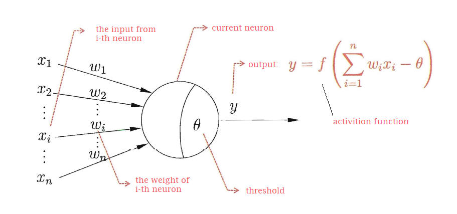
M-P neuron model was invented by McCulloch and Pitts in 1943 as shown in figure.1. In this model, the neuron receives the information from N neurons. The information from these neurons is passed with their corresponding connection weights. There is a threshold in current neuron to compare the input with itself to determine this information will put out or not. If passing the threshold, the activation function is then used to process the output. 

(Figure.1. M-P neuron model)

2) Logistic Sigmoid

logistic sigmoid or sigmoid function is one of common-used activation fucntions in neural networks. It is defined in the form:

The graph of sigmoid function is: the definition domain is R, the range of f(x) is (0,1).

(Figure.2. sigmoid function graph)

3. Error Backpropagation

1) Function

Backpropagation is a method used in artificial neural networks to tune the parameters by distributing the global error backward throughout the network's layers, more specifically, all weights and thresholds. As inputs go forwards, the way that the error propagate backward to the parameters is called error backpropagation, the shorthand for "the backward propagation of errors".

(Figure.3. Error BackPropagation)

2) Parameter Learning

From the previous description, the backpropagation algorithm is generally, directly applied to shallow structure networks. Here, I take a single hidden layer neural network (shown in Figure.4.) as the example to show the working process of the BP.  

(Figure. 4 BP network)

The aim of the BP is to minimize the cumulative error (generally subject to the training set). Assume that there are m sub-sets in the training set. The cumulative error can be displayed as Formula.1:

(Formula 1.)

Standard BP only updates the parameters for one sub-set. it means for m sub-sets, the standard BP will be employed individually for them. Of course, there is another way called cumulative BP, which updates the entire training set at a time. Since their principles are the same, I only consider the standard BP here. Moreover, as for basic neuron model (as shown in Figure.1), I just skip it assuming the readers already have a basic understanding of that. 

For the k-th sub-set (X_k, Y_k) of the training set, the error E_k is usually presented by the mean square error (MSE), shown in formula.2. 

(Formula. 2)

where X_k stands for the input of the k-th sub-set and Y_k stands for the output of this BP network (shown in Figure. 4).  Formula. 3 shows the output of this network.

(Formula. 3 the output of this BP network)

Minimizing the E_k is an optimization problem to find the Minimum, and the gradient descent method (referring to my past post) will be used to adjust the parameters. So each parameter will use v ←v+∆v to update themselves. Use the partial derivative of E_k subject to ∆w_hj to update ∆w_hj and we have: where, η is the learning rate or the step length.

(Formula. 4)

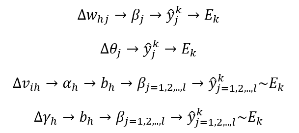
The chain rule of computing the partial derivative is very important in this process. To let you more understand that, I give a brief affection chain as shown in Formula. 5.

(Formula. 5 Chain rule of partial derivative)

Based on that, we can get the update formulas of all parameters as shown below. the standard BP use sigmoid function as its activation function, and this function has the characteristic like below.

(Formula .6 sigmoid)

(Formula. 7 for ∆w_hj)

(Formula. 7 for ∆θ_j)

(Formula. 9 ∆v_ih)

(Formula. 10 ∆γ_h)

3. Conclusion

the BP here is more a rule than a model since all networks will use BP to tune their parameters. Since the BP algorithm is used to distribute backward the real error of loss function which is a measure of how good a prediction model does in terms of being able to predict the expected outcome, to all parameters. It is a supervised learning algorithm. So a training set with the input and output should be given. 

The activation function here I introduced is the sigmoid function, actually, there are some other activation methods, like ReLU. The traditional BP algorithm is difficult to be applied to deep multi-layer neural networks is partly due to the sigmoid function which faces the divergence problem (or vanishing gradient problem) when the error propagates backward in multi hidden layers. In order to solve this issue, many ways have been put up, like the RMB (an unsupervised learning algorithm) that I will present in the next post and ReLU. ReLU is another activation function used in BP, but compared to sigmoid, it avoids the problem that sigmoid faces when applied to deep networks. ReLU will be analyzed in a post of this series later.