Short-Term/Time Fourier Transform, STFT

1. Introduction

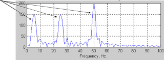
In a time-invariant system, the signal is stationary as shown in figure 1.1. Figure 1.1 is a signal with three frequency component. From this figure, we can see the sampling frequency of this signal is stable. After Fourier transform, we will get three frequency components on the frequency-amplitude system as shown in figure 1.3 all the time since the sampling frequency fs is fixed.

Figure.1.1 stationary signal

Figure.1.2 The FT of a stationary signal

In a time-varying system, the signal is non-stationary as shown in figure 1.3. From this figure, we can see the sampling frequency fs of this signal varies along the time. After FT, we do get three frequency components as shown in figure 1.4. However, we have no information about where these frequencies are located in time as the sampling frequency fs changes along with time.

Figure.1.3 non-stationary signal

Figure.1.4 The FT of a non-stationary signal

Therefore:
For the time-invariant system, the main function of Fourier analysis is to extract the frequency information, which is independent to sampling time and sample length (only meeting Nyquist–Shannon sampling theorem), of the given sequence. But for the time-varying system, different sampling time and sample length have different frequency distributions. Apart from the frequency distribution, we are also interested to know the frequency distribution along with time. Then we can locate a specific frequency at a specific time. Obviously, traditional Fourier analysis e.g. FT, DFT is not useful for analyzing this sort of time-variant, non-stationary signals. In order to provide simultaneous time and frequency location, Short-Term/Time Fourier Transform (STFT) is put forward. STFT is a powerful general-purpose tool for audio signal processing.

Figure 1.5 the relationship between STFT and time&freqency

2. Background

2.1 Convolution

what is the convolution?
From a Mathematical point of view, the convolution is a rule that defines the operation between two functions or consequences.
From a Physical point of view, the convolution stands for the modulation of a system with respect to a certain  Physical quantity or input.
From a signal point of view, the convolution shows the response way of a linear system affecting the input signal. The output is the convolution of a system impact on the input signal. It is in the form of integration. Since convolution is widely-used in signal processing, I step it from the signal aspect.

• Function Transformation

Assume I(t) stands an impact function of a system. t is the time. If the graph of I(t) is shown below.
In figure 2.1, the black part is the original graph of I(t). Given an impact at t=0, the effect of this impact is fading along the time. Our interest here is about how this impact propagates to the epoch t=T. Therefore, we ignore the left, shadowed part and only consider the right part. According to the aforesaid, the propagation of this impact at t=0 is a declining process to the t=T. Then following this rule, if giving another impact at t=T, its graph will be like the graph in red as shown. Let's focus on the interval [0, T]. Obviously, it is not right if we use the impact at t=0 to replace the impact at t=T since the impact amplitude is stronger with the time closer to the epoch launching impact. That is why each epoch should have its own impact. One thing that needs to know is the impact at each epoch will propagate to the time area ahead of current epoch but not propagate to the time area after this epoch.
What is the relationship between the black and red functions subject to [0, T]?
tips: the impact function is symmetry.
Randomly select a point in the black graph, (t1, I(t1)) and a point in the red graph, (t2, I(t2)) and t1+t2=T, according to the symmetry, I(t1) should equal to I(t2). Then we have I(t1)=I(t2)=I(T-t1). Therefore, I(t)=I(T-t).

Figure 2.1

Depending on the link between the function and its graph, we can transfer the black graph to the red graph via two steps: 1) rotate I(t) 180 degree around the Y-axis to get I(-t); 2) move I(-t) to the right at the distance of T to get I(T-t). the process is shown in figure 2.

Figure 2.2

The example taken here is a symmetry graph. Actually, this transformation is also suitable for the non-symmetry graph. You only need to replace the shadowed part with any other forms of graphs.

• Continuous Convolution Definition

If f1(t) and f2(t) are two functions with (-∞, +∞) as their definition domain, the integration S(t), expressed in formula 1, is the convolution of f1(t) and f2(t),  f1(t) * f2(t).

Formula 1. The definition of convolution

If assign some restrictions for the f1 and f2, we have:

Formula 2. 

For the linear time-invariant system, the definition domain of f1 and f2 is as the restriction iii, namely, effective interval [0,  +∞]. Thus, the definition domain of the convolution S(t) of the linear time-invariant system is [0, t].
Let's link the convolution and function transformation together. The function f1(τ) can be viewed as the signal input, and f2(t-τ) can be viewed as the impulse function at epoch t. As the aforesaid, it is not right to directly replace f2(t-τ) with f2(τ) since the impact function is launched at the epoch t. Besides, the impact at t will propagate to the time area ahead of the t, namely, it will affect all input signal ahead of that time. We need to sum them up as the integration. This progress is also called discrete convolution since the input signal needs to be individually separated to be able to be processed by computers. The discrete convolution is shown later. (The meaning of convolution in signal processing, you can also refer to the section 2.2 Finite Impulse Response filter)

• Convolution Features

Distribution law:

Formula 3. 

Combination law:

Formula 4. 

Exchange law:

Formula 5. 

Convolution Differential:

Formula 6. 

Convolution Integral:

Formula 7. 

Convolution related to Singularity function:

Formula 8. 

• Discrete Convolution Definition

In order to make the signal can be processed by computers, it needs to be individually separated. For discrete signal, we have discrete convolution:

Similar to continuous convolution, discrete convolution also have those features as the continuous convolution has. In particular, the differential and integral of discrete convolution are as follows:
Discrete Convolution Differential:

Formula 9.

Discrete Convolution Integral:

Formula 10.

2.2 Finite Impulse Response (FIR) filter

A finite impulse response (FIR) filter is a filter whose impulse response (or response to any finite length input) is of finite duration because it settles to zero in finite time. This is in contrast to infinite impulse response (IIR) filters, which may have internal feedback and may continue to respond indefinitely (usually decaying).
FIR filters are widely used in signal processing. The main function of it is to filter out those unwanted signal and keep the useful signal.
For a FIR filter, the type of processing can be expressed in the form:

Figure 2.1 discrete-time direct-type FIR filter of order N

Where z−1 is called unit delay. h(N-n) is called the coefficient of this FIR filter and stands for the value of the impulse response at the N-n instant. x(n) is the input and y(n) is the output. N is the filter order and an N-order filter has (N+1) terms from 0.
The value of y(n) can be displayed as Formula 11.

Formula 11.

 Actually, this computation is also known as discrete convolution. According to the feature of convolution, h(x)=h(T-x) and h(x) is a symmetry function with the center axis x=T/2. More specifically,  h(x)=±h(T-x), for h(x)=h(T-x), it is a even symmetry and for  h(x)=-h(T-x), it is an odd symmetry. Generally, N is an even number.

Now, we know how a FIR filter works. Let's have a deep look at the difference between IIR and FIR. According to their definition, the IIR is infinitely approaching to zero but never equals. Compared to the IIR, FIR can equal to zero in a fast way. So what are the meanings of these two forms?

Figure 2.4 the difference between IIR and FIR

As the aforesaid, at a certain instant x=0, the system gives an impulse. The effect of this impulse is similar to the reduction of energy which is fading away along the time but it never disappears. That is exactly the feature of the IIR. Theoretically, the output signal is the sum of all input multiplying their coefficients from the impulse which is infinite. However, an infinite signal cannot be processed by machines. We have to turn it into a finite fashion. So we replace the IIR with the FIR. Consequently, our problem is how to design a FIR which minimizes the effect due to this replacement. This process is also called FIR filter design. The h(k) in formula 11 is a filter. 

2.3 Window Function

FIR design filters are almost entirely restricted to discrete-time implementations. The design techniques for filters are based on directly approximating the desired frequency response of the discrete-time system. The simplest method for FIR design is called the Window method. Literally,  the Window method is a window-shape FIR filter as shown in figure 2.5. The wider of the window, the more samples will be included. For a time-invariant system, the signal is stationary so the window size doesn't affect the frequency analysis. But for a time-variant system, the window size should be set carefully as it has a big impact on the frequency analysis.

Figure 2.5

Now that we know why we need a window function, then I will show you some commonly used window functions. Figure 2.6 gives you an overview of these functions' graphs. M is the size of the window. There are five window functions in all: Rectangular, Hamming, Hanning, Blackman, Bartlett. 

Figure 2.6 the graph of commonly used window functions

These function equations of these windows are shown in figure 2.7.

Figure 2.7: function equations

From these function equations and graphs, we can see that these window functions have symmetry feature and its symmetry center is M/2.
The features of the Window function are:

• Symmetry: the symmetry center is n=M/2. M is the length of the window. 
• w(n-t)=w(t-n). Obviously, moving right the graph at a distance of t, w(n-t), equals to rotating 180° of the graph around the symmetry axis firstly and then moving right distance t, w(t-n).

3. Model Analysis

• Definition

Figure 3.1 gives the definition of STFT.

Figure 3.1 STFT Formula 

In the discrete time case, the data to be transformed could be broken up into chunks or frames (which usually overlap each other, to reduce artifacts at the boundary). Each chunk is Fourier transformed, and the complex result is added to a matrix, which records magnitude and phase for each point in time and frequency. This can be expressed as:

Figure 3.2

likewise, with signal x[n] and window w[n]. In this case, m is discrete and ω is continuous, but in most typical applications the STFT is performed on a computer using the Fast Fourier Transform, so both variables are discrete and quantized. 

• Time

The aim of STFT is to provide both time information and frequency information. Here, the Window function has two tasks: one is to act as a window-shape FIR filter; the other is to provide the time information. As shown in Figure 3.1, we can see the Window function is centered at t=t' (t' is a certain time epoch). If the size of a window is M, then the duration of this window is T=M/fs (fs is sampling frequency). Via Fourier transform, we can get the frequency information of the samples in this window. Then sliding the window, we can transform the next window. 

One thing we need to know is that STFT cannot provide a very specific time information but time interval. 

• Frequency

Once given a time epoch, STFT turns into FFT. After Fourier transform, the frequency within the current window is extracted. More information please refer to FFT.   

• Spectrogram 

Apart from the frequency and time information, the magnitude of corresponding frequencies is also should be presented. So we often use a spectrogram to achieve this. A spectrogram is a visual representation of the spectrum of frequencies of sound or other signals as they vary with time. Spectrograms are sometimes called sonographies, voiceprints, or voicegrams.
A common format is a graph with two geometric dimensions: one axis represents time or RPM, the other axis is frequency; a third dimension indicating the amplitude of a particular frequency at a particular time is represented by the intensity or color of each point in the image.

Figure 3.3 an example of Spectrogram

Generally, the magnitude squared of the STFT yields the spectrogram representation of the Power Spectral Density of the function:

Figure 3.4

• Features

As shown in Figure 3.5, the wide window has good frequency resolution and poor time resolution. But the narrow window has good time resolution and poor frequency resolution. Because given a finite sequence, the length of a window determines the number of segments. The wide window includes more samples resulting in more sub-frequencies. But the duration of this window will be longer as the M is larger. (here the window size should meet Nyquist–Shannon sampling theorem.)

Figure 3.5 Comparison of STFT resolution. Left has better time resolution, and right has better frequency resolution.

Figure 3.6 Comparison of windows with different sizes.

Window should be narrow enough to make sure that the portion of the signal falling within the window is stationary.

Very narrow windows do not offer good localization in the frequency domain.

• Application

In practical, both FFT and STFT need sliding window technique to process a long sequence. For FFT, we don't need to provide a window function. About the size of a window, we often consider the duration of target activities as well as the sampling theorem. In order to increase the related accuracy, there is a proportion of overlap between the two windows.   
For STFT, the length of a window should be narrow enough to make sure that the portion of the signal falling within the window is stationary. As the aforesaid, very narrow windows do not offer good localization in the frequency domain. Therefore, we need to make a balance.

4. Conclusion

In this post, I briefly introduced the time-invariant and time-variant systems, the definition of convolution, the IIR filter and the FIR filter and STFT in detail. The structure of this post is as shown below.

Figure 4.1 structure.

© 2018 Bang Wu All Rights Reserved