You Raise Me Up

Wednesday, 13 March 2019

【toturial】import function of python

There are many ways to import modules or packages.

regular imports
from __ import __
relative imports
optional imports
local imports

regular imports

import single module or package

import sys

import sys as system

import multi-modules or packages
import os, sys, time

import sub module or package
import urllib.error

from import

from is used when you only want to import one part of a module and package

from functools import lru_cache
from os import path, walk, unlink
from os import uname, remove

from os import (path, walk, unlink, uname, 
                remove, rename)
from os import path, walk, unlink, uname, \
                remove, rename

from is used when you want to import all of a module and package

from os import *

relative imports

Case 1:

Given a file structure like this

we want to import subpackage 1 and subpackage 2 in the top __init__.py

from . import subpackage1

from . import subpackage2

But it will occur a problem like

The reason is that this subpackage is not initialized.

The solution to this problem is to add two commands before using "from . import subpackage1"

import subpackage1

import subpackage2

from . import subpackage1

from . import subpackage2

Then in both subpackage1 and subpackage2, there generates a file directory named __pycache__ for each other.

Once generating this file, next time you can directly use

from . import subpackage1

from . import subpackage2

You may notice the file in the directory __pycache__ is __init__....

what does that mean?

let's go on and look back later

If we want to import module_x and module_y in __init__.py under subpackage1

from . import module_x

from . import module_y

the same problem will occur

Then we use the method described above, as

import module_x

import module_y

from . import module_x

from . import module_y

Then you will find

__init__.cpython-37.pyc

module_x.cpython-37.pyc

module_y.cpython-37.pyc

So that looks like a registration, once appearing in this directory, then you can use them.

Case 2:

If we want to use my_package as well as its packages and modules inside.

For example, we create a testpackage, test.py

So the way of import my_package is:

import sys

sys.path.append('C:/Users/acw393/Dropbox/SecondYearResearch')

import my_package

from my_package import module_a

Attention, the path should be the upper directory of my_package

This case is very useful when you use local modules!!

Here is an example to use local modules! (attention: this case is that target module and current runfile are not in the same file directory)

the location of the target module

__init__.py is the initial function of the whole module. if you import seglearn, the __init__ will automatically run.

But I want to use this module named seglearn in a file,

What we should do is to:
1) add a sys path of current target module into system environment:
__init__.py :
import sys
sys.path.append('C:/Users/Bang/Dropbox/SecondYearResearch/Seglearn-revised')
import seglearn

2) add the same thing at any runfile where you directly use seglearn.
import sys
sys.path.append('C:/Users/Bang/Dropbox/SecondYearResearch/Seglearn-revised')
import seglearn

Here, we can know, if we create a module (which should have __init__.py to initially run all sub-modules), we only need to add following code in the __init__.py of that module.
import sys
sys.path.append(path): path means the file directory where the defined module is.
import name_definedmodule

then add the same code in the file you want to import.

Optional imports

It is used when you wish to use a certain module by priority or use a backup when the target module doesn't exist.

try:
    # For Python 3
    from http.client import responses
except ImportError:  # For Python 2.5-2.7
    try:
        from httplib import responses  # NOQA
    except ImportError:  # For Python 2.4
        from BaseHTTPServer import BaseHTTPRequestHandler as _BHRH
        responses = dict([(k, v[0]) for k, v in _BHRH.responses.items()])

try:
    from urlparse import urljoin
    from urllib2 import urlopen
except ImportError:
    # Python 3
    from urllib.parse import urljoin
    from urllib.request import urlopen

Local imports

import sys  # global scope

def square_root(a):
    # This import is into the square_root functions local scope
    import math
    return math.sqrt(a)

def my_pow(base_num, power):
    return math.pow(base_num, power)

if __name__ == '__main__':
    print(square_root(49))
    print(my_pow(2, 3))

circular imports

# a.py
import b

def a_test():
    print("in a_test")
    b.b_test()

a_test()

import a

def b_test():
    print('In test_b"')
    a.a_test()

b_test()

Shadowed imports

import math

def square_root(number):
    return math.sqrt(number)

square_root(72)

Tips for establishing your own module and package

1. import all you need in __init__.py. This is a good habit for a programmer.

Reference

http://codingpy.com/article/python-import-101/

Tuesday, 12 March 2019

[Research] An introduction of Conda, Git, Pip

1. Introduction

Anaconda is a release version of python, of which features are supporting Linux, Mac, Windows and providing environment and package management ability. It is very convenient to switch between multi-version python. In Anaconda, Conda provides Package, dependency and environment management for any language—Python, R, Ruby, Lua, Scala, Java, JavaScript, C/ C++, FORTRAN

Conda is an open source package management system and environmental management system that runs on Windows, macOS and Linux. Conda quickly installs, runs and updates packages and their dependencies. Conda easily creates, saves, loads and switches between environments on your local computer. It was created for Python programs, but it can package and distribute software for any language.

Conda as a package manager helps you find and install packages. If you need a package that requires a different version of Python, you do not need to switch to a different environment manager, because conda is also an environment manager. With just a few commands, you can set up a totally separate environment to run that different version of Python, while continuing to run your usual version of Python in your normal environment.

Apart from conda, pip is the package installer for Python. You can use pip to install packages from the Python Package Index and other indexes.

Git is a free and open source distributed version control system designed to handle everything from small to very large projects with speed and efficiency.

So in this post, I will introduce the difference between those tools.

2. Anaconda

Figure 1. Anaconda installation directory

The general way to install the Anaconda is to download the software on its website. Once choosing the python version and x86/x64, you can directly download and install in your computer. Figure 1 shows the installation directory on my computer.

We see in the main directory, there includes [env] and [python]. The reason why I mention these two is it can show the main feature of the Anaconda in environment management. [python] in this directory means a chosen version python and spyder are already installed. So if you directly choose Spyder from the start. you are using the pre-defined type of python. In this default python, there are many packages already installed there. You can directly import and use it.

Figure 2. package already installed in default.

We can view this default as the base(root) environment. Then I will introduce the environment management of the tool conda.
First I will show you how to create a new environment as shown above:
1) open Anaconda Prompt
2) $conda create --name testpy python=3.6
3) $conda activate testpy
4) $conda install spyder
5) $spyder

Now this testpy has been created under [env] and spyder is also installed. Comparing figure 1 and 3, you will find them almost the same. But they work independently. The packages they use are also independent. That means the packages used by default spyder are not used by testpy. Testpy need to install by itself.

Figure 3. testpy installation directory

Figure 4. package installed for testpy.

3. pip

Generally, conda is mainly used for environment management. Of course, you can also use it to install or uninstall some packages. But here, I want to introduce the tool, pip.

pip is used for install or uninstall packages for python (spyder).
The format of language is: pip install package_name; pip uninstall package_name
attention: there are two ways to directly use pip commands. 1) directly use the command windows [Home + R]; 2) the second is to use Anaconda Prompt and #(base) model
The location of downloading packages is:

Figure 5. Location of installed package

As mentioned before, we created another environment testpy, and we intalled spyder for this environment. we also can use pip to install packages for this environment. The installed location is shown below.

Figure 6. Location of installed package for testpy

In this environment, if we want to use pip install, we need to enter Anaconda Prompt and $(testpy) model.

conda is also used for install and uninstall packages, but it needs to use Anaconda Prompt.
For default python (spyder), we use $(base) model, for a specific environment like testpy, we use $(testpy).

the commands like:
(testpy) C:\Users\acw393>conda install -n testpy filterpy
(base) C:\Users\acw393>conda install numpy

4. Git

Here is a Chinese tutorial: https://www.cnblogs.com/tugenhua0707/p/4050072.html

Saturday, 2 March 2019

[Research] The principle of Bayes Filter

The principle of Bayes Filter

1. Introduction

The Bayesian filter is an important class of filters. It is widely used in object tracking, robot positioning and so on. And it is the basis of filters like the Kalman Filter (KF), Extended Kalman Filter (EKF), Information Filter (IF) and Particle Filter (PF). It is a type of filter using prior knowledge and causal knowledge (also called likelihood) to deduce posterior knowledge. This process can be displayed by Bayes Theorem:

Equation 1. Bayes Theorem

Actually, there are two types of filters, parametric filters (e.g. Kalman filters, Information filters) and non-parametric filters (e.g. histogram filter, discrete Bayes Filter, Particle Filter).

The feature of parametric filters is that the system status can be expressed by parametric models. That means the posterior information of the system is explicit. The most common parametric model is Gauss model (corresponding distribution is normal distribution). The parameters used are mean and variance.
The feature of non-parametric filters is the system is independent to the posterior information. Unlike the parametric filters whose posterior information can be analytically displayed by models (e.g. Gauss model), non-parametric filters use finite samples to approximate posterior probability.

As I said before, both parametric filters and non-parametric filters are using the framework of Bayes Theorem. Combine prior information (prediction model) and causal information (measurement model) to deduce the posterior information. So it is quite beneficial to have a good understanding of Bayes Filter. Therefore, this post will focus on the principle and some related background of the Bayes Filter.

2. Background

2.1 Probability and Bayes Theorem

P(X=xi) means the probability when X equals xi
For discrete variables, P(⋅) is called the probability mass function. e.g. p(X) = {0.1, 0.2, 0.7}
For continuous variables, P(x∈(a,b)) =∫p(x)dx is called the probability density function

Figure 2.1.1 the probability density function

Joint Probability: p(X=x and Y=y)=p(x,y), is called the Joint Probability Density Distribution. If X and Y are independent, p(x,y)=p(x)p(y).
Conditional Probability: p(X=x|Y=y) means given Y=y, compute the probability when X=x. p(x|y)=p(x,y)/p(y); p(x,y)=p(x|y)p(y)=p(y|x)p(x). Specially, if X is independent to Y, p(x|y)=p(x).
Law of total probability:

Equation 2. law of total probability

Bayes Theorem: as shown in Equation 1 above. From it, we can see p(y) is independent to p(x|y). So p(y) can be viewed as a normalization factor of which function is to keep p(x|y) under 1.

Equation 3. normalization factor

2.2 Discrete-time Markov Chain

A discrete-time Markov chain is a stochastic model describing a sequence of possible events in which the probability of each event depends only on the state attained in the previous event. This process can be displayed by:

Equation 4. The feature of the probability of Discrete-time Markov Chain4

There are a few features of Markov Chain:

memorylessness for first-order Markov Chain: From Equation 3, we know the current status is only dependent on the most previous status.
First-order and n-order: Generally, we talk about the first-order Markov Chain. But Markov chain also has a version for high-order. High-order MC is an extension of first-order MC. The form is like this: we see compared to first-order MC, n-order MC is dependent on the n most previous state, which means n-order MC has a memory.

Equation 5. First-order and n-order of MC

Transition probability: is the probability going from state i to state j in single-step transition or multi-step transition. e.g.

Equation 6. Transition probability

Transition Matrix: If the state space is finite, the transition probability distribution can be represented by a matrix, called the transition matrix. Similarly, the transition matrix has a single-step transition, multi-step transition or mix. Here is an example of a single-step transition:

Equation 7. Transition matrix

Connectivity: every two states are connected. some of them are directly connected and others are not directly connected where we can use transition matrix to connect them.
Stationary distribution: given an arbitrary state Π = [π(1), π(2),..., π(j)], Σπ(j) = 1; if Π(i) = Π(j)Pij, we call it stationary distribution. The code showing below give you an example to validate this distribution. You will find that the state in stationary distribution is independent on the initial state. That means, only Pij will affect this stationary distribution.

#python code

p=np.array([[0.65,0.28,0.07],[0.15,0.67,0.18],[0.12,0.36,0.52]])

p2 = np.array([[0.21,0.68,0.11]])

#p2 = np.array([[0.286, 0.489, 0.225]])

for i in range(20):

print("index", i)

p2 = np.dot(p2,p)

print(p2)

index 0

[[0.2517 0.554 0.1943]]

index 1

[[0.270021 0.511604 0.218375]]

index 2

[[0.27845925 0.49699556 0.22454519]]

index 3

[[0.28249327 0.49179188 0.22571485]]

index 4

[[0.28447519 0.48985602 0.22566879]]

index 5

[[0.28546753 0.48909735 0.22543512]]

index 6

[[0.28597071 0.48878278 0.22524651]]

index 7

[[0.28622796 0.488645 0.22512704]]

index 8

[[0.28636017 0.48858171 0.22505812]]

index 9

[[0.28642834 0.48855152 0.22502014]]

index 10

[[0.28646357 0.4885367 0.22499973]]

index 11

[[0.28648179 0.48852929 0.22498892]]

index 12

[[0.28649123 0.48852554 0.22498323]]

index 13

[[0.28649612 0.48852362 0.22498026]]

index 14

[[0.28649865 0.48852263 0.22497872]]

index 15

[[0.28649996 0.48852212 0.22497791]]

index 16

[[0.28650064 0.48852186 0.22497749]]

index 17

[[0.286501 0.48852173 0.22497728]]

index 18

[[0.28650118 0.48852166 0.22497716]]

index 19

[[0.28650128 0.48852162 0.22497711]]

p=np.array([[0.65,0.28,0.07],[0.15,0.67,0.18],[0.12,0.36,0.52]])

#p2 = np.array([[0.21,0.68,0.11]])

p2 = np.array([[0.286, 0.489, 0.225]])

for i in range(20):

print("index", i)

p2 = np.dot(p2,p)

print(p2)

index 0

[[0.28625 0.48871 0.22504]]

index 1

[[0.2863738 0.4886001 0.2250261]]

index 2

[[0.28643612 0.48855613 0.22500776]]

index 3

[[0.28646783 0.48853751 0.22499466]]

index 4

[[0.28648407 0.4885292 0.22498672]]

index 5

[[0.28649243 0.48852533 0.22498224]]

index 6

[[0.28649675 0.48852346 0.22497979]]

index 7

[[0.28649898 0.48852253 0.22497849]]

index 8

[[0.28650014 0.48852207 0.2249778 ]]

index 9

[[0.28650073 0.48852183 0.22497744]]

index 10

[[0.28650104 0.48852171 0.22497725]]

index 11

[[0.2865012 0.48852165 0.22497715]]

index 12

[[0.28650129 0.48852161 0.2249771 ]]

index 13

[[0.28650133 0.4885216 0.22497707]]

index 14

[[0.28650135 0.48852159 0.22497706]]

index 15

[[0.28650136 0.48852158 0.22497705]]

index 16

[[0.28650137 0.48852158 0.22497705]]

index 17

[[0.28650137 0.48852158 0.22497705]]

index 18

[[0.28650138 0.48852158 0.22497704]]

index 19

[[0.28650138 0.48852158 0.22497704]]

Convergence: Whatever the state space is finite or infinite. Markov chain will be into a stationary distribution after many steps transition. And this stationary distribution is only associated with the transition matrix, not the intial state. Thus, Morkov chain has a feature of convergence. if initial state: X0 ∼ π0(x); state i: Xi ∼ πi(x), πi(x) = πi−1(x)P = π0(x)P^n. Once reaching stationary distribution, it has: Xn ∼ πn(x) = π(x); Xn+1 ∼ π(x); Xn+2 ∼ π(x). Namely: π(i)Pij = π(j)Pji for all i, j. So we call π(x) is the stationary distribution and Xn, Xn+1 and Xn+2 are the samples under stationary distribution. This feature is quite important and it is the basis of MCMC(Markov Chain Monte Carlo).

2.3. Sampling

Statistics and probability:

Figure 2.3.0 Statistics and probability

Probability, we also call prior information; statistics, also called posterior. In the real world (computer world), we only use statistics to evaluate theoritical model. That's why we need sampling to evaluate the probabilitic model. Using a finite number of randomly sampled points to compute a result is called sampling. The idea is simple. Generate enough points to get a representative sample of the problem, run the points through the system you are modeling, and then compute the results on the transformed points.

For example, if we want to compute Pi: we can draw a square with side length 2 and a circle with radius 1 inside of the square. And we generate a set of uniformly distributed random points within the square and count how many fall inside the circle. The area of the circle is computed as the area of the square times the ratio of points inside the circle vs. the total number of points. Finally, we know that A=πr2, so we compute π=A/r2.

Fig 2.3.1 compute π

As for probability density function (PDF), the equation is:

It also equals the area under the curve. It is easy to compute the integral with definite equation/formula. But for many curves, they are hard to analytically describe, not to mention integrate it like below:

Fig 2.3.2 Arbitrary curve

In this situation, we can use sampling methods to compute the integral. e.g. let x falls in [a,b], then building a box which wraps the curve [a,b]. Then generating a set of uniformly distributed random points within the box and count how many fall under the curve, and get the area under the curve.

Then a question is How to generate samples under a distribution p(x)? This method is the so-called Monte Carlo sampling.

2.4. Monte Carlo Sampling

Monte Carlo sampling was invented by Stanley Ulam at Los Alamos National Laboratory to allow him to perform computations for nuclear reactions which were unsolvable on paper. we can use Monte Carlo to compute the probability density of any probability distribution.

There is an important sampling method called MCMC(Markov Chain Monte Carlo). As described before at section of Markov chain, we call π(x) is the stationary distribution and Xn, Xn+1 and Xn+2 are the samples under stationary distribution. One beautiful thought is set the stationary distribution as our target, p(x). Once the system entering into stationary distribution, all samples are satisfied to p(x). Then we can design the transition matrix Q for this Markov chain to make the samples generated satisfied to p(x).

Of course, this is just a brief description of the principle of MCMC. For more details you can refer to.

MCMC now becomes the most commonly used method to generate samples satisfied certain p(x). For example, in Numpy.random, there are gauss distribution, uniform distribution, and some other distributions. We can call these API for convenience. Besides, we also can use PyMC3.

3. Bayes Inference and Bayes Filter

3.1 Bayes Inference

Bayes Theorem is the basic framework of Bayes inference as shown in Equation 3, using prior information and likelihood to deduce posterior.

In many applications, we need to fuse multi-source information to deduce the system status. Here is the formula to fuse multi-source information. We see the basic rule is under the Bayes Theorem framework, using the law of total probability to do factorization.

Equation 8. fusion of multi-source information

Here x is the system status, y.z are two measurements. we can view them as the measurement at different epochs. Assume z is the previous measurement and y is the current status. P(x|y,z) means the posterior probability of current status based on measurements y,z. p(y|x,z) means the conditional probability given the current status x and last measurement z. p(x|z) means the conditional probability of current status x given the measurement z. and p(y|z) means the conditional probability of current measurement given the last measurement.

Bayesian recursion formula:
We have introduced how to use Bayes Theorem to deduce system status. However, sometimes, we need to use the previous multi-status to infer. That's the Bayesian recursion formula.

Equation 9. Bayesian recursion formula

From Equation 9, Bayes recursion formula has the feature of Markov Chain. Use the conditional probability to make the transition between statuses.

Here is an example to practice Bayes Inference.

3.2 Bayes Filter

In practical, apart from the self-measurement, a system would be affected by a dynamic environment. For example, the system affects itself or outside action affects this system. We can build a scene like this. for a robot, it can move one step at each epoch. To get the accurate status of the system, we need to measure to evaluate system status. So there are two sections, section 1: the system itself can change from current status to next status.We also called it prection. Section 2: we can measure the real-time status of the system. The aim of the Bayes filter is to fuse the prediction and measurement to update the system status.

Assume u is the action (e.g. moving one step), x′ is the status before this action, x is the status after this action. So P(x|u,x′) means the posterior status after the action u. The form is:
(The effect of action towards status is displayed by the status transition model. here is an example.)

Equation 10. P(x|u,x′)

Then we have a framework for Bayes filter:

Given the prior probability of system status, p(x)
Given the system measurement z and action u at 1 to t: dt = {u1, z1,..., ut, zt}
Given the measurement model/probability p(z|x)
deduce the posterior probability p(x|u,x′). namely, Bel(xt)=P(xt|u1,z1…,ut,zt)
Assumption 1: Markov Characteristic, namely, The status at t is determined by the status at t−1 and action at t. The measurement at t is only related to the status at t. In other words, zt is the outer calibration of the system status, ut is the energy to predict system status.

Figure 3.2.1 Assumption 1

Assumption 2: observation noisy (for zt) and model noisy (for xt) are independent.
Assumption 3: Assume other environment factors unchanged.

So Bayes Filter is:

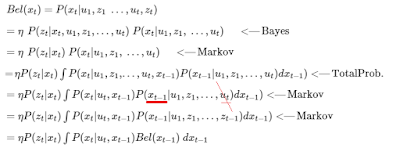
Equation 11 (1)

Equation 11(2). Bayes Filter

We see Equation 11 (1), the first step is the expansion of Bayes Theorem. The inference of η is shown in Equation 11 (2). And step 2 is using the Markov characteristic, namely, zt is determined by xt. Step 3 is using the law of total probability to get xt-1. Step 4 is still the Markov feature, xt is determined by xt-1 and ut. Similarly, due to Markov feature, xt-1 is not related to ut.

In a nutshell, there are two steps: ∫P(xt|ut,xt−1)Bel(xt−1)dxt−1 is using xt-1 and ut to get the prediction status of xt. And ηP(zt|xt) is used to update the xt using zt.

Algorithm flow:

Figure 3.2.2 Algorithm flow

From this flow, we see there are two parts: update part and prediction part. When there is just an action (e.g. advancing one step, moving into next epoch), the system will be self-updated in a predicted manner. when doing a measurement, z, the system will fuse measurement, z, and prediction to update the status.

4. Practice: Bayes Filter

Here is an example to show how Bayes filter works.

Assume a system has 10 different statuses. In the beginning, the probability of each status is equal. So the initial status of this system is belief = [0.1, 0.1, 0.1, 0.1, 0.1, 0.1, 0.1, 0.1, 0.1, 0.1].
Assume there is no measurement. If the system moves into another status. then we need to make a prediction for system status. Currently, belief1 would equal belief. Of course, this is a special example, if the initial belief is [.35, .1, .2, .3, 0, 0, 0, 0, 0, .05]. That means, we think the system is more likely to be the first position. Then if the system moves on, the belief1 would be [.05, .35, .1, .2, .3, 0, 0, 0, 0, 0]. This process is a prediction.
Then we have a list of possible measurement, hallway = np.array([1, 1, 0, 0, 0, 0, 0, 0, 1, 0]). Where 1 means that position is a door. 0 means that position is a wall. Taking tracking a dog walking in a corridor as an example, one time of measurement may indicate it stops at a door or a wall. When z=1,=>door; z=0, =>wall. The initial probability for measurement should be: [0.1, 0.1, 0.1, 0.1, 0.1, 0.1, 0.1, 0.1, 0.1, 0.1].
Assume current measurement z equals 1 with a probability 75%. That means a 25% chance of wall. The probability for measurement should be p(z|x) = [0.3, 0.3, 0.1, 0.1, 0.1, 0.1, 0.1, 0.1, 0.3, 0.1]. =likelihood
Then the prior probability of this system is [0.1, 0.1, 0.1, 0.1, 0.1, 0.1, 0.1, 0.1, 0.1, 0.1]. we have a measurement z = 1; then we can update the status by using p(x|z) = p(z|x)p(x)/normalization. so the posterior probability of status should be: [0.03, 0.03, 0.01, 0.01, 0.01, 0.01, 0.01, 0.01, 0.03, 0.01]. As its sum doesn't equal 1, we need to normalization. So we let p(x|z)/sum(p(x|z)) = p(x|z)/0.16 = [0.1875, 0.1875, 0.0625, 0.0625, 0.0625, 0.0625, 0.0625, 0.0625, 0.1875, 0.0625].
The source code is shown below:

def lh_hallway(hall, z, z_prob):

""" compute likelihood that a measurement matches

positions in the hallway."""

try:

scale = z_prob / (1. - z_prob)

except ZeroDivisionError:

scale = 1e8

likelihood = np.ones(len(hall))

likelihood[hall==z] *= scale

return likelihood

def update(likelihood, prior):

posterior = prior * likelihood

return normalize(posterior)

def normalization(pdf)

pdf /= sum(np.asarray(pdf, dtype=float))

return pdf

hallway = np.array([1, 1, 0, 0, 0, 0, 0, 0, 1, 0])

belief = np.array([0.1] * 10)

likelihood = lh_hallway(hallway, z=1, z_prob=.75)

posterior = update(likelihood, belief)

posterior = normalization(posterior)

5. Conclusion

This post covered Bayes Theorem, Markov Chain, Monte Carlo, Bayes Inference and Bayes Filter. The link between those is:

Figure 5.1

We see, the framework of Bayes inference is to use likelihood and prior information to deduce the posterior. It is intuitive as sometimes we can't direct get the posterior information. We need to generate samples to approximate probabilities. The method we used is Monte Carlo. Actually, Monte Carlo means the way how to generate samples to approximate probabilities. This method is already applied in many random data applications. We may not know the principle of Monte Carlo, you need to know its function.

And the framework of Bayes Filter includes two parts: one part is the prediction, one is the update. If there is no outer measurement, the transition of system status will be implemented by prediction. If there is a measurement, Bayes filter will combine prediction and measure to compute the posterior and update.

Both Bayes Inference and Bayes Filter use the feature of Markov Chain, namely, the current status is only related to the last status.

Bayes Filter is a kind of non-parametric filter as it doesn't directly evaluate the parameter. It uses a sampling method to approximate the posterior information. But these two parts (prediction and update) is the basis for other filters, e.g. Kalman filter, Extended Kalman filter. Particle filter and so on. Apart from Bayes Filter, Particle filter and Histogram filter are also non-parametric filters.

Kalman filter is a parametric filter as its probability is Gauss model. We only need to evaluate the mean and variance of the status to obtain the model. Then directly use this model to infer the transition of the system.